Head-to-Head Effects
Matchup effects are a common idea in tennis commentary. It is the thing at the heart of comments like ‘her game matches up well’ against her opponent. One way to think of a matchup effect is as a surprising head-to-head, when results go against what the overall ability of both players would have us expect. Do such effects exist? And are they substantial enough that they matter when it comes to making better predictions about tennis results?
I’ve been working on predicting wins in tennis for some time. Whenever I’ve had a chance to talk about the method with tennis insiders, there is always one question I know will come up (if only predicting match results was as easy to forecast!). That is, whether I account for head-to-head.
In one sense, any method that includes the historical results of a player is accounting for head-to-head. But I know that this isn’t exactly what the question is getting at. The question really comes down to matchup effects and the particular edge one player might have over a specific opponent that goes beyond what their ability would predict, factors like style or intimidation, for example.
Most prediction methods (and I’ve explored many over the years) assume that players abilities are transitive. That is, if player A is two times greater in overall ability than players B and C, than his win expectations in a match against B and C should be equal. Matchup effects throw a wrench into the transitive property and effectively act like an interaction term, where the overall abilities of players can’t in themselves explain the results of their matches against each other.
That description gets us on track to how we might identify the presence of head-to-head effects. Suppose we have our favourite approach for predicting the chance player $i$ wins a match against player $j$ that doesn’t account for matchup effects (so this might exclude bookmaker odds, for example). Call this expectation $\hat{p}_{ij}$. A basic model to account for head-to-head is:
$$logit[P(W_{ij} = 1)] = \beta_0 + \beta_1 \hat{p}_{ij} + \alpha_{ij}$$
The parameter $\alpha_{ij}$ is the key here. It is an unknown constant for the specific matchup that adjusts our expectations when $\hat{p}_{ij}$ assumes abilities are transitive.
What is a Typical Head-to-Head?
Before we fit such a model, even before we decide whether to use likelihood-based or Bayesian methods, we need to decide which data to use. Just considering the men’s game, do we include Futures? Challengers? or limit it to ATP events only?
The answer comes down to where most repeat clashes are happening. We know that tennis is a pyramid, with the size of the competitive pool shooting upward the lower down you go down the tournament tier. We might suspect that, for this reason, players at the Challenger level, for example, will not often build up substantial head-to-heads against other players on the tour.
But what does the data actually show?
Considering all matches played in the past 10 years at the Challenger level having any head-to-head turns out to be quite. If we consider how likely it is that two players drawn at random from the competitor pool (anyone who ever competed in a Challenger event or better during this period) have played each other in competition before, the chance is just 2 out of 100. The chance that any random pairs has a match history of 3 or more is a 3 in 1000 chance. We might have already thought that the 53-match rivalry of Nadal and Djokovic was unusually long but this summary tells us that even a 3-match history is a 1% of 1% event in the professional game.
| Head-to-Head Sample Size | Frequency (+ Challengers) | Frequency (- Challengers) |
|---|---|---|
| 0 | 98.4% | 96.0% |
| 1 | 1.2% | 2.5% |
| 2 | 0.3% | 0.8% |
| 3+ | 0.1% | 0.7% |
Even if we drop Challenger events, the break down doesn’t change dramatically. Among players competing primarily at the tour-level, the chance is still under 1% that any pair among them will have played 3 matches or more over a 10 year period.
Why does any of this matter for estimating head-to-head effects? If there are many cases of player-opponent matchups with a single match, it can impact the accuracy of estimates of the head-to-head effects, pulling all effects closer to zero than would be the case with a less sparse sample.
The infrequency of lengthy head-to-heads also suggests that any adjustment for them (if such were warranted) is unlikely to have a substantial improvement in prediction performance more generally. The number of matches in a season that would involve players with an even moderate match history would be few. But we will come back to this later.
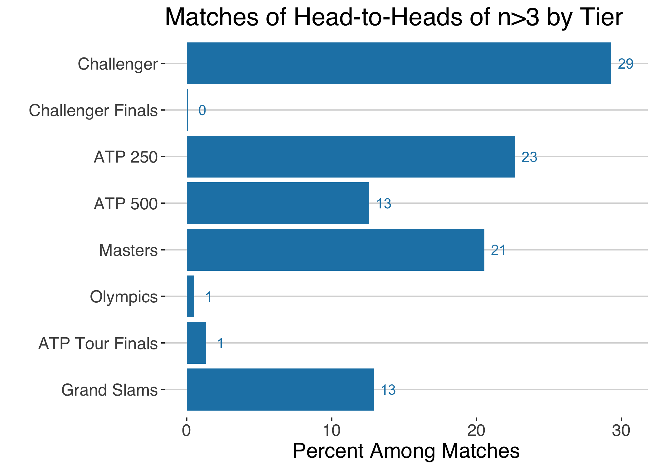
We have seen that having played more than 3 matches against an opponent is an unusually long history compared to the norm. Among matches played for players in this ‘long’ rivalry subgroup, 1 in 3 of the matches happened at the Challenger level, 1 in 4 at the 250 level, and 1 in 5 at the Masters level.
Head-to-Head Effects
Given the preponderance of singleton head-to-heads, I will examine matchup effects among player-opponent pairs with a history of 2 or more matches prior to 2018 at the Challenger level or above (reserving 2018 and 2019 matches for out-of-sample testing).
For the $\hat{p}_{ij}$, I will use a surface-adjusted Elo rating1. This is a dynamic transitive model that also accounts for surface specialty. In using this as the prediction covariate, the aim is for the head-to-head to capture any intransitive effects no explained by the overall ability or surface preferences of the players.
When a logistic mixed model was fit to these matchups, the standard deviation for the player-opponent random effect was $\sigma = 0.40$, suggesting evidence of matchup effects. When we look at the conditional means for the specific effect estimates $\hat{\alpha}_{ij}$ 1 in 6 would imply an adjustment in predictions of 15% or more. Another indication of statistically meaningful head-to-head effects.
The chart below is a forest plot of the 100 biggest head-to-head effects found in the men’s sample. The effect is expressed in terms of the factor you would multiply the standard odds by for these players to account for the head-to-head effect. The player who benefits from the head-to-head effect is the one on the left in the x-axis labels. Larger dots indicate the effects with greater relative certainty.
There are a lot of interesting things to pick out of these effects (and it is only a sample of the 100 largest ones!). At the very top of the chart we see a cluster of head-to-heads involving Stan Wawrinka and Tomas Berdych, their own head-to-head being the one with the largest effect overall. These two have faced each other 16 times in their career with Wawrinka leading 11 to 5; 10 times since 2010 with Wawrinka dropping just 1 match. My surface-adjusted ratings show that Berdych was ahead of Wawrinka for all of their last 10 matches, though they have also been close, differing by no more than 50 points at any one occasion. That would make Wawrinka’s edge over Berdych look surprisingly lopsided.
It is a similar story with Wawrinka’s matchup against Cilic. Wawrinka has won all of their 8 most recent matches (they’ve faced each other 14 times overall) despite Cilic surpassing Wawrinka in the player ratings in 2016 and 2017.
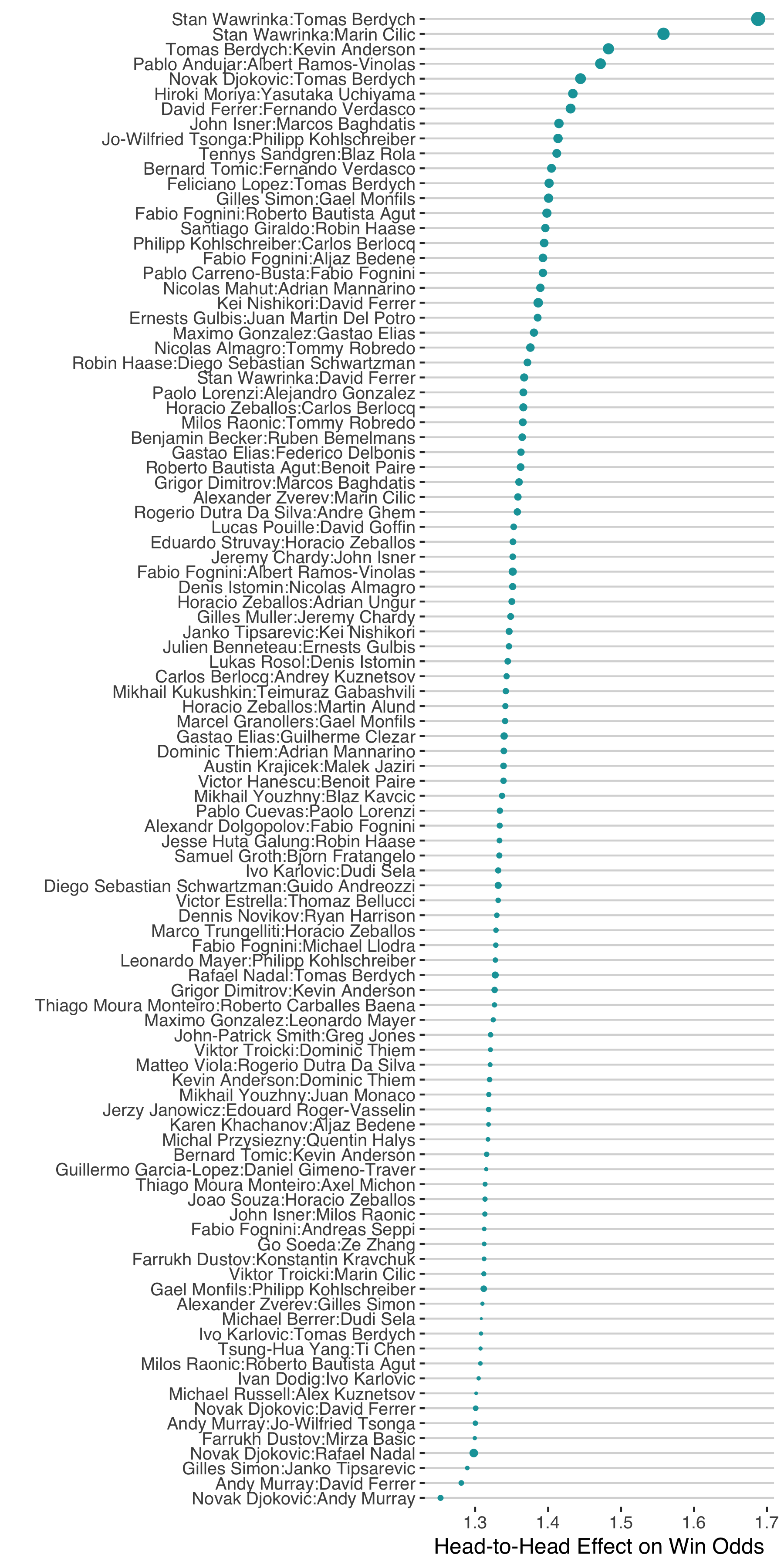
There are several players who pop up in multiple of the biggest head-to-head effects. Fabio Fognini features 7 times in the list, having the benefit of the matchup class for 5 of these, with the biggest edge being over Roberto Bautista Agut.
Berdych is the next most frequently occurring player in the list with 6 head-to-heads, which is the same number that Horacio Zeballos appears in. David Ferrer comes up in a total of 5 of the head-to-heads and is at the wrong end of the stick for 4 of the 5 (vs Andy Murray, Novak Djokovic, Stan Wawrinka, and Kei Nishikori). Ferrer is an interesting case because he is often considered one of the best players who always came short against the Big 4. This tells us that the head-to-head effects could also come up when a player has a ceiling effect in their ability and not necessarily playing style clashes alone.
There are some head-to-heads people might have expected to see in the top 100 that don’t appear. Rafael Nadal and Roger Federer is one. The head-to-head effect in this case gives a 7% boost to Rafael Nadal, not insignificant but also not as big as some might have thought. I think this can be explained by the fact that most of Nadal’s wins over Federer have been on clay (13 of 23) where his surface-adjusted rating would have explained that record.
The clash between Federer and Wawrinka gets a bigger head-to-head effect, with Federer getting a 20% boost in his odds when facing Wawrinka. That would make Federer’s recent win over Wawrinka at Indian Wells that much less surprising.
Another interesting matchup with relevance for Indian Wells was Gael Monfils win over Philipp Kohlschreiber. With Kohlschreiber coming off a massive upset over Novak Djokovic, many might have thought it was his time to go deep. Monfils was going to be a hard opponent for anyone but the head-to-head effect suggest it is an especially tricky matchup for Kohli, whose matchup against Monfils puts him in the top 100 and would give him a 30% disadvantage against Monfils.
Prediction Improvement
We don’t even have to apply the head-to-head correction to know that it isn’t going to move prediction improvement upward for the majority of matches. There are just too few matches between players who have played each other at all in the past to get any benefit from such an adjustment. But that doesn’t mean that the correction isn’t valuable.
The nature of tennis means that the biggest rivalries will tend to be between the most well-known players. The three biggest rivalries in the dataset used in this post are Nadal v Djokovic, Federer v Djokovic, and Djokovic v Murray. So, although the occurrence of big n head-to-heads are rare, they are high impact matches when they occur.
So if we focus just on matches where head-to-head might matter, what do we find? Using matches from 2018-2019 as the test data, there were 754 that involved players with a head-to-head history of more than 3 matches. The overall change in prediction accuracy from the standard prediction to one with the head-to-head correction was negligible for this group.
| Match Type | Number of Matches | Standard Prediction Accuracy | +H2H Prediction Accuracy |
|---|---|---|---|
| Matchups with n>3 Match History | 754 | 66.6% | 66.7% |
| Subgroup of Close Matches | 233 | 54.9% | 55.4% |
| Subgroup where H2H Changed Predicted Winner | 21 | 47.6% | 52.4 % |
If we look at the subset among these that were close, where the standard prediction was somewhere between 40% and 60%, does the correction perform any better? The accuracy was 55.4% with head-to-head effects versus 54.9%, which is an improvement but one that might not hold up with repeated sampling, given that it is based on 233 matches.
The final subgroup we consider are the cases where the consideration of head-to-head actually reversed the favoured player (the player with >50% win expectation). There were only 21 matches of this type, a small sample, but one that showed the biggest difference in the use of head-to-head or not, with a 5 point gain in accuracy for the prediction with the head-to-head correction.
Because this last subgroup is an especially interesting one, and a group where the correction for matchup has the biggest impact, I’ve plotted each of those matches below. The result and predictions are all with respect to the first player in the matchup.
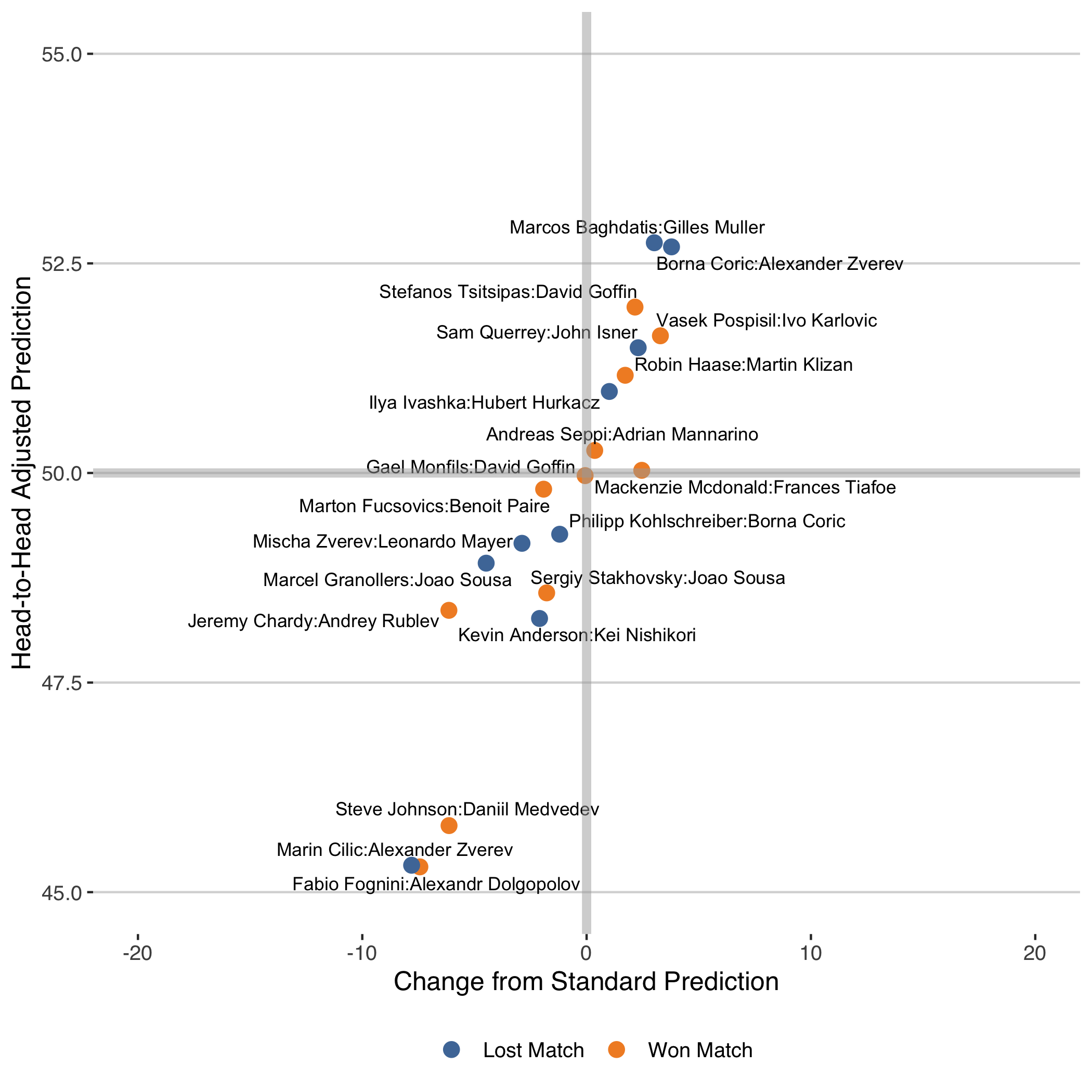
The chart shows, for example, that Stefanos Tsitsipas would have gotten +2 percentage points toward his win prediction when he faced David Goffin this year in Marseille owing to the head-to-head correction, a match he did win.
Although there were more changes in the right direction, there were plenty in the wrong direction as well. Marin Cilic’s loss to Alexander Zverev at the 2018 ATP World Tour Finals is a prime example. The head-to-head correction pulled the match much more in favour of Cilic (53% versus 45%) but the match went to Zverev in that instance.
Style versus Head-to-Head
Even with some evidence of improvement in close matches with lengthy head-to-heads, small sample sizes still make adjusting for head-to-head difficult. The most obvious way to overcome this would be to look at grouping players by their style of play, which would allow us to draw strength from players with similar styles to estimate matchup effects. It is the obvious path but how to go about defining playing style if far from clear. For now, adjustment for specific head-to-heads has some merits and also reveals both expected and surprising results about the biggest matchup effects in the game.
-
Technically, the Elo rating system supposes a linear relationship between the log odds for the win and the rating difference of the player. However, using the probability transformation of the prediction has some advantages in terms of numerical stability of the model. But the choice of transformation doesn’t have a huge impact on the results either way. ↩︎